Chapter 4 Opportunities for advancing field

Up to now has been an overview of the techniques in deep learning that have been successfully and commonly implemented in sequential classification problems. This chapter will be devoted to new efforts of solving problems associated with the aforementioned methods. In addition to being a survey of the current state of the art it will also identify potential avenues for new research that could enhance our ability to work with sequential data subjected to various constraints.

4.1 What to do with all those parameters

An issue with not just sequence-based deep learning, but the field as a whole, is how large models are. For instance: VGGnet (Simonyan and Zisserman (2014)), the second place winner of the 2014 ImageNet competition and an extremely common model to use for image recognition tasks, has 138 million parameters to tune. Going by the rule of thumb from Frank Harrell’s book “Regression Modeling Strategies” (Harrell Jr (2015)) of 10-20 observations per parameter in our model, this is an issue, especially given the size of the data-set that the VGGnet model was trained on was only one million images¹⁰.

Even simple neural nets have a large number of parameters. A model with just a single hidden layer taking a ten dimensional input and a hidden layer of ten neurons performing binary classification would have (with bias parameters included) \((10*11) + (10*11) + (2*11) = 242\) parameters to tune.

4.1.1 Theory backed methods for choosing model architectures

How then, did the VGGnet model achieve an accuracy of 93% on the test set? The answer lies in the fact that data is not shared over parameters in the same way it is in regression models. This stems from the fact that each layer’s parameters are using as their input the output from the previous layer, and thus data are being reused. While it does not appear that this means we only need to count the parameters in the first layer, it does mean that deep learning models need to be thought of differently than traditional regression based models in terms of parameter complexity(^It also points to the advantages of deep neural nets over wide ones, a topic considered more deeply in Goodfellow, Bengio, and Courville 2016, chap. 13.).

As of yet, there is no solid theoretical explanation of exactly what the data to parameter relationships are in deep neural networks, and thus there are no concrete guidelines to model construction. Difficulties in ascertaining these guidelines seems in part due to the non-convex optimization routines used for the models.

The combination of the lack of theory and the computational time needed to perform traditional grid-search techniques for tuning layer numbers/size suggest the potential for very impactful research in this area.

4.1.2 Runtime on mobile hardware

Another impact of having extremely large models is they take a long time to not only train, but to be used to predict as well. If deep learning models are to be brought to mobile devices such as smart phones or watches the models need to be scaled down in terms of their size and run time complexity substantially. Efforts towards this have been successful with models such as SqueezeNet (Iandola et al. (2016)) drastically reducing the number of parameters compared to traditional convolutional networks, while still maintaining a good level of accuracy in ImageNet prediction performance. In addition, certain forms of penalization such as \(L_0\) penalization can be applied to ‘thin out’ a network by forcing certain weights to drop to zero and then throwing them out (Louizos, Welling, and Kingma (2017)), all while performing a single run of stochastic gradient descent, eliminating the need to do costly re-training of the network after dropping weights.

Great opportunity lies the development of objective and rigorous methods of eliminating unnecessary parameters in models. Approaches such as regularization are promising as are the evaluation of model response to techniques such as dropout (Srivastava et al. (2014)) where by neurons are randomly dropped during forward propigation in training in an effort to build robust prediction pathways. An analysis of a model’s response to certain neuron’s being dropped may indicate the potential for sparsity inducing techniques.

4.2 Inference

A great source of confusion for many statisticians when reading literature in the deep learning world is that in many cases the same words have different meanings. “Inference” is a good example of this. To a statistician inference means the dissection of the inner workings of the model: what parameters are used to make predictions and how confident are we in those parameters. In deep learning, inference typically refers to the use of a model for prediction. There are a few things that stand in the way of traditional inference in deep learning models.

4.2.1 Peering into the black box

Often it is common to hear people refer to deep neural networks as “black box predictors.” This meaning simply that data goes in and the model performs some uninterpretable transformations to that data and returns its prediction. While in giant models such as VGGnet may make this seem like the case, it is actually quite possible to see what is going on within a neural network, just the quantity of information to understand is too high to fully comprehend it in its raw form.

The desire for traditional inference in the statistical sense is a limiting goal. Having a parameter estimate and its uncertainty works well when models are single-stage linear combinations of the data, but neural networks, and arguably the world, does not usually work in linear combinations. Traditional inference has relied on making (hopefully) non-impactful simplifications of the true nature of the system being modeled in order for it to fit the framework of linear models.

With deep learning we have a system theoretically capable of modeling any function of data and we should take advantage of that. If the model objectively performs well, we should perform the simplification on the explanation side, rather than the model side. How exactly this is done is not a solved issue (and may never be), but some early examples include the work of visualizing the intermediate layers in computer vision models (Olah, Mordvintsev, and Schubert (2017)): investigating the features learned by neural networks can provide great insight into the way it parsing the signals in the data.

4.2.2 Generative Adversarial Networks

One approach that allows simultaneously attempting to train a better model, but also understanding the workings of the model is a class of deep learning models called “generative adversarial networks” (or GANs)(Goodfellow et al. (2014)). GANs train two separate neural networks in tandem: a generator and a discriminator. The job is for the generator to construct fake examples of some training set and the discriminator’s job is to decide if the example is a real observation or a generated one. These models have shown remarkable results in terms of image generation such as those recently presented by NVIDIA 4.1 (Karras et al. (2017)).

The output of a generative adversarial network trained on a database of celebrity faces. Both faces seen are entirely generated by the model and show that it learned to a very precise degree, what constitutes a 'face.'

Figure 4.1: The output of a generative adversarial network trained on a database of celebrity faces. Both faces seen are entirely generated by the model and show that it learned to a very precise degree, what constitutes a ‘face.’

The output produced by the generator model of GANs effectively show what the descriminator model is ‘seeing’ when it chooses to classify something as a given class. For instance, an over-fit model may classify a house as a house because it sees a lot of the color blue in the sky. If that was the case a GAN would simply return a blue canvas when asked to generate a house¹¹.

Recently, a team at ETH Zurich used GANs on time series data taken from hospital records (Esteban, Hyland, and Rätsch (2017)) and found that GANs could be used successfully on these data to generate realistic looking medical data, suggesting that the model was learning underlying patterns well¹².

4.2.3 Causality problems

While much of deep learning is not currently focused on uncovering causal pathways¹³, given the ability of these models to generalize so well, it is worth exploring the issue more. One area of concern with the models mentioned is the temporal order of data. For instance, in convolutional methods for sequence classification, often the convolutions are allowed to explore not only back in time, but also forward in time to classify at a given instance. The same goes with a class of RNNs that we didn’t discuss but have proved successful: the bi-directional RNN. In this case the RNN’s hidden state path travels not only forward in time, but also backwards.

These models that can see both backward and forward in time often perform better than their omni-directional counterparts. For instance, in speech the “au” phoneme may indicate an ‘e’ or an ‘a’ in a word, but it only becomes clear after the end of the word is heard which value it is. However, the flow of causality is forward in time, so these models explicitly violate this.

Potentially fitting a model that has the ability to see both forward and reverse temporal dependencies and then investigating the dependencies that were discovered by both directions could provide some insight into this. For instance, if the backwards in time component of the RNN found that the administration of some drug was a strong signal that high blood-pressure would later occur, but not the reverse direction the relationship could warrant further experimental exploration of causality potential. It would be necessary to make sure that the patterns discovered were not due to residuals from the reverse-time predictors, but this could be done by forcing the model to ‘forget’ those patterns and seeing if our forward-time trends remain.

4.3 Small or sparse data

Deep learning has come to be almost synonymous with ‘big data.’ Most of the groundbreaking work tends to come out of large companies with massive data-sets and near-infinite compute power to fit their models. This has left the area of deep learning corresponding to small data relatively unexplored. We have already seen that deep learning models seem to use their parameters more efficiently than traditional statistical methods, but that is clearly not without limit. The following are a brief survey of a few techniques for dealing with small or sparse (meaning a large portion missing labels) data.

4.3.1 Bayesian deep learning

As we have seen, a neural network is essentially a series of stacked linear models with static non-linear transformations applied. Much like we can fit a regression model in a Bayesian context, we can fit a deep neural network with Bayesian techniques. To do so, each tuneable parameter is simply provided a prior (usually a normal centered at zero) distribution and the posterior distribution is determined the same as any other Bayesian model. Usually variational inference techniques are used instead of sampling techniques such as Hamiltonian Monte Carlo due to the size of the models (Blundell et al. (2015)).

Bayesian neural networks have been shown to perform more efficiently on small data-sets than traditional models (Srivastava et al. (2014)). In addition, some generative models such as autoencoders (see section below) have shown subjectively better results from Bayesian implementations than standard implementations (Kingma and Welling (2013)).

4.3.2 Semi-supervised methods

In many circumstances the data may not be small as a whole, but the number of observations that have labels for the desired prediction are. An example of this is activity tagging data. For each day twenty four hours of time-series data are gathered on the subject, but often when asked to tag the data they only tag specific instances of activities, leaving much of the day blank. In addition it is often infeasible to ask them to label every day of their data.

Another example comes from EHR based studies. Many times these studies rely on using physicians to perform chart reviews in order to construct their training and test sets. This is a costly and time consuming procedure.

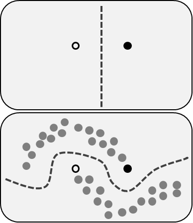
Visual example of how adding unlabeled data can provide valuable information about the shape of the data valuable for classification. Image taken from Wikipedia.

Figure 4.2: Visual example of how adding unlabeled data can provide valuable information about the shape of the data valuable for classification. Image taken from Wikipedia.

There are various approaches to dealing with this sparse data issue. A very promising avenue is the preliminary fitting of an unsupervised model on the data, followed by a supervised learning model using features learned by the unsupervised model

Say we wished to classify sentiment of a corpus of text, but only had labels of sentiment for a small subsection of the text. First an unsupervised model would be fit to all of the data. For instance a model trained to predict the next word in a sentence. This unsupervised model would learn to map the text at a given time-point to some latent-space that holds information about the next word and most likely sentiment as well. Tthe final layer of the word prediction model that maps that latent-space to the next word is removed and replaced with a new layer that fits the form of our desired classification (in this case a binary outcome of “happy” or not). This new model is then trained on the labeled data with the weights of the lower-layers either frozen at their values from the unsupervised step or simply initialized at them.

This approach of unsupervised pre-training has been shown to yield great improvements in the performance of sequence models (Zhu (2005)).

Other methods of performing semi-supervised learning include training the model on available labels, then using the trained model to classify the unlabeled data and then retraining the model treating those labels as the true values. Surprisingly this method does almost always yield improvements over not using any unlabeled data(Zhu (2005)).

Exploration of the operating characteristics of semi-supervised learning scenarios could be a valuable contribution to areas of research such as electronic health records. An example of potential impact: a pseudo power calculation could be performed at the outset of a modeling effort. This would help the researchers optimize time and money by informing how many labeled examples needed to be collected. In addition, efforts to extend the performance benefits of semi-supervised learning could allow models to be fit to domains where they were previously not able to be due to difficulties in gathering labels for data.

Bengio, Yoshua, and Paolo Frasconi. 1994. “Credit Assignment Through Time: Alternatives to Backpropagation.” In Advances in Neural Information Processing Systems, 75–82.

Berndt, Donald J, and James Clifford. 1994. “Using Dynamic Time Warping to Find Patterns in Time Series.” In KDD Workshop, 10:359–70. 16. Seattle, WA.

Blundell, Charles, Julien Cornebise, Koray Kavukcuoglu, and Daan Wierstra. 2015. “Weight Uncertainty in Neural Networks.” arXiv Preprint arXiv:1505.05424.

Cai, Xindi, Nian Zhang, Ganesh K Venayagamoorthy, and Donald C Wunsch. 2007. “Time Series Prediction with Recurrent Neural Networks Trained by a Hybrid Pso–EA Algorithm.” Neurocomputing 70 (13). Elsevier: 2342–53.

Cho, Kyunghyun, Bart Van Merriënboer, Dzmitry Bahdanau, and Yoshua Bengio. 2014. “On the Properties of Neural Machine Translation: Encoder-Decoder Approaches.” arXiv Preprint arXiv:1409.1259.

Esteban, Cristóbal, Stephanie L Hyland, and Gunnar Rätsch. 2017. “Real-Valued (Medical) Time Series Generation with Recurrent Conditional Gans.” arXiv Preprint arXiv:1706.02633.

Goh, Gabriel. 2017. “Why Momentum Really Works.” Distill. doi:10.23915/distill.00006.

Goodfellow, Ian, Yoshua Bengio, and Aaron Courville. 2016. Deep Learning. MIT press.

Goodfellow, Ian, Jean Pouget-Abadie, Mehdi Mirza, Bing Xu, David Warde-Farley, Sherjil Ozair, Aaron Courville, and Yoshua Bengio. 2014. “Generative Adversarial Nets.” In Advances in Neural Information Processing Systems, 2672–80.

Graves, Alex. 2012. Supervised Sequence Labelling with Recurrent Neural Networks. Vol. 385. Springer.

Graves, Alex, Marcus Liwicki, Horst Bunke, Jürgen Schmidhuber, and Santiago Fernández. 2008. “Unconstrained on-Line Handwriting Recognition with Recurrent Neural Networks.” In Advances in Neural Information Processing Systems, 577–84.

Graves, Alex, Abdel-rahman Mohamed, and Geoffrey Hinton. 2013. “Speech Recognition with Deep Recurrent Neural Networks.” In Acoustics, Speech and Signal Processing (Icassp), 2013 Ieee International Conference on, 6645–9. IEEE.

Harrell Jr, Frank E. 2015. Regression Modeling Strategies: With Applications to Linear Models, Logistic and Ordinal Regression, and Survival Analysis. Springer.

Hochreiter, Sepp, and Jürgen Schmidhuber. 1997. “Long Short-Term Memory.” Neural Computation 9 (8). MIT Press: 1735–80.

Hochreiter, Sepp, Yoshua Bengio, Paolo Frasconi, Jürgen Schmidhuber, and others. 2001. “Gradient Flow in Recurrent Nets: The Difficulty of Learning Long-Term Dependencies.” A field guide to dynamical recurrent neural networks. IEEE Press.

Hornik, Kurt, Maxwell Stinchcombe, and Halbert White. 1989. “Multilayer Feedforward Networks Are Universal Approximators.” Neural Networks 2 (5). Elsevier: 359–66.

Iandola, Forrest N, Song Han, Matthew W Moskewicz, Khalid Ashraf, William J Dally, and Kurt Keutzer. 2016. “SqueezeNet: AlexNet-Level Accuracy with 50x Fewer Parameters And< 0.5 Mb Model Size.” arXiv Preprint arXiv:1602.07360.

Jose M. Sanchez, MD, BS Brandon Ballinger, MD FHRS Jeffrey E. Olgin, MD MPH Mark J. Pletcher, PhD Eric Vittinghoff, BA Emily Lee, BA Shannon Fan, et al. 2017. “Detecting Atrial Fibrillation Using a Smart Watch - the mRhythm Study.” In Heart Rhythm Scientific Sessions. Heart Rhythm Society.

Karras, Tero, Timo Aila, Samuli Laine, and Jaakko Lehtinen. 2017. “Progressive Growing of Gans for Improved Quality, Stability, and Variation.” arXiv Preprint arXiv:1710.10196.

Kheradpisheh, Saeed Reza, Masoud Ghodrati, Mohammad Ganjtabesh, and Timothée Masquelier. 2016. “Deep Networks Can Resemble Human Feed-Forward Vision in Invariant Object Recognition.” Scientific Reports 6. Nature Publishing Group: 32672.

Kingma, Diederik P, and Max Welling. 2013. “Auto-Encoding Variational Bayes.” arXiv Preprint arXiv:1312.6114.

Krizhevsky, Alex, Ilya Sutskever, and Geoffrey E Hinton. 2012. “Imagenet Classification with Deep Convolutional Neural Networks.” In Advances in Neural Information Processing Systems, 1097–1105.

LeCun, Yann, and others. 1989. “Generalization and Network Design Strategies.” Connectionism in Perspective. Zurich, Switzerland: Elsevier, 143–55.

Lin, Tsungnan, Bill G Horne, Peter Tino, and C Lee Giles. 1998. “Learning Long-Term Dependencies Is Not as Difficult with Narx Recurrent Neural Networks.”

Louizos, Christos, Max Welling, and Diederik P Kingma. 2017. “Learning Sparse Neural Networks through L\(_{0}\) Regularization.” arXiv.org, December. http://arxiv.org/abs/1712.01312v1.

Mao, Junhua, Wei Xu, Yi Yang, Jiang Wang, Zhiheng Huang, and Alan Yuille. 2014. “Deep Captioning with Multimodal Recurrent Neural Networks (M-Rnn).” arXiv Preprint arXiv:1412.6632.

McCulloch, Warren S, and Walter Pitts. 1943. “A Logical Calculus of the Ideas Immanent in Nervous Activity.” The Bulletin of Mathematical Biophysics 5 (4). Springer: 115–33.

Melis, Gábor, Chris Dyer, and Phil Blunsom. 2017. “On the State of the Art of Evaluation in Neural Language Models.” arXiv.org, July. http://arxiv.org/abs/1707.05589v2.

Mikolov, Tomas, Ilya Sutskever, Kai Chen, Greg S Corrado, and Jeff Dean. 2013. “Distributed Representations of Words and Phrases and Their Compositionality.” In Advances in Neural Information Processing Systems, 3111–9.

Minsky, Marvin, Seymour A Papert, and Léon Bottou. 1969. Perceptrons: An Introduction to Computational Geometry. MIT press.

Nair, Vinod, and Geoffrey E Hinton. 2010. “Rectified Linear Units Improve Restricted Boltzmann Machines.” In Proceedings of the 27th International Conference on Machine Learning (Icml-10), 807–14.

Olah, Chris, Alexander Mordvintsev, and Ludwig Schubert. 2017. “Feature Visualization.” Distill. doi:10.23915/distill.00007.

Ordóñez, Francisco Javier, and Daniel Roggen. 2016. “Deep Convolutional and Lstm Recurrent Neural Networks for Multimodal Wearable Activity Recognition.” Sensors 16 (1). Multidisciplinary Digital Publishing Institute: 115.

Pinheiro, Pedro, and Ronan Collobert. 2014. “Recurrent Convolutional Neural Networks for Scene Labeling.” In International Conference on Machine Learning, 82–90.

Ravi, Nishkam, Nikhil Dandekar, Preetham Mysore, and Michael L Littman. 2005. “Activity Recognition from Accelerometer Data.” In Aaai, 5:1541–6. 2005.

Rosenblatt, Frank. 1958. “The Perceptron: A Probabilistic Model for Information Storage and Organization in the Brain.” Psychological Review 65 (6). American Psychological Association: 386.

Rumelhart, David E, Geoffrey E Hinton, and Ronald J Williams. 1986. “Learning Representations by Back-Propagating Errors.” Nature 323 (6088). Nature Publishing Group: 533–36.

Rush, Alexander M, Sumit Chopra, and Jason Weston. 2015. “A Neural Attention Model for Abstractive Sentence Summarization.” arXiv Preprint arXiv:1509.00685.

Sabour, Sara, Nicholas Frosst, and Geoffrey E Hinton. 2017. “Dynamic Routing Between Capsules.” In Advances in Neural Information Processing Systems, 3857–67.

Salimans, Tim, Jonathan Ho, Xi Chen, Szymon Sidor, and Ilya Sutskever. 2017. “Evolution Strategies as a Scalable Alternative to Reinforcement Learning.” arXiv.org, March. http://arxiv.org/abs/1703.03864v2.

Shickel, Benjamin, Patrick Tighe, Azra Bihorac, and Parisa Rashidi. 2017. “Deep Ehr: A Survey of Recent Advances on Deep Learning Techniques for Electronic Health Record (Ehr) Analysis.” arXiv Preprint arXiv:1706.03446.

Simonyan, Karen, and Andrew Zisserman. 2014. “Very Deep Convolutional Networks for Large-Scale Image Recognition.” arXiv Preprint arXiv:1409.1556.

Srivastava, Nitish, Geoffrey E Hinton, Alex Krizhevsky, Ilya Sutskever, and Ruslan Salakhutdinov. 2014. “Dropout: A Simple Way to Prevent Neural Networks from Overfitting.” Journal of Machine Learning Research 15 (1): 1929–58.

Sussillo, David. 2014. “RANDOM Walks: TRAINING Very Deep Nonlin-Ear Feed-Forward Networks with Smart Ini.” arXiv Preprint arXiv 1412.

Waibel, Alex, Toshiyuki Hanazawa, Geoffrey Hinton, Kiyohiro Shikano, and Kevin J Lang. 1989. “Phoneme Recognition Using Time-Delay Neural Networks.” IEEE Transactions on Acoustics, Speech, and Signal Processing 37 (3). IEEE: 328–39.

Williams, Ronald J, and Jing Peng. 1990. “An Efficient Gradient-Based Algorithm for on-Line Training of Recurrent Network Trajectories.” Neural Computation 2 (4). MIT Press: 490–501.

Williams, Ronald J, and David Zipser. 1989. “A Learning Algorithm for Continually Running Fully Recurrent Neural Networks.” Neural Computation 1 (2). MIT Press: 270–80.

Wu, Yonghui, Mike Schuster, Zhifeng Chen, Quoc V Le, Mohammad Norouzi, Wolfgang Macherey, Maxim Krikun, et al. 2016. “Google’s Neural Machine Translation System: Bridging the Gap Between Human and Machine Translation.” arXiv Preprint arXiv:1609.08144.

Yu, Fisher, and Vladlen Koltun. 2015. “Multi-Scale Context Aggregation by Dilated Convolutions.” arXiv Preprint arXiv:1511.07122.

Zhou, Chunting, Chonglin Sun, Zhiyuan Liu, and Francis Lau. 2015. “A c-Lstm Neural Network for Text Classification.” arXiv Preprint arXiv:1511.08630.

Zhu, Xiaojin. 2005. “Semi-Supervised Learning Literature Survey.” Citeseer.

References